多变量的线性回归

n: 特征(features) 数量
m: 训练集数量
$x^{(i)}$:

表示一条训练数据的向量
i is an index into the training set
So
- x is an n-dimensional feature vector
- $x^{(3)}$ is, for example, the 3rd training data

$x^{(j)}_i$: The value of feature j in the ith training example

例如，当 n=4 时:

$h_θ(x) = θ_0 + θ_1x_1 + θ_2x_2 + θ_3x_3 + θ_4x_4$

For convenience of notation, $x_0$ = 1, 所以最后的特征向量的维度是 n+1，从 0 开始，记为”X”，
则有：

$h_θ(x)=θ^TX$

$θ^T$: [1 * (n+1)] matrix

多变量的梯度下降

Cost Function

$J(θ_0, θ_1, ...,θ_n) = \frac1{2m}\sum_{i=1}^{m}{(h_θ(x^{(i)}) - y^{(i)})^2}$

Gradient descent

Repeat {

$θ_j = θ_j - α\frac\partial{\partial J(θ_0, θ_1, ...,θ_n)}$

}

every iterator

θj = θj - learning rate (α) times the partial derivative of J(θ) with respect to θJ(…)
We do this through a simultaneous update of every θj value

$\frac\partial{\partial J(θ_0, θ_1, ...,θ_n)}$ $= \frac1m * \sum_{i=1}^{m}{(h_θ(x^{(i)}) - y^{(i)})}*x_j^{(i)}$

Gradient Decent in practice

Feature Scaling

假设只有 $x_1$,$x_2$ 两个变量，其中：$x_1\in(0,2000), x_2\in(1,5)$，则最后的 J(θ) 图形是一个椭圆，在椭圆下用梯度下降法会比圆形要耗时更久，So we need to rescale this input so it’s more effective，有很多方式，一种是将各个 feature 除以其本身的最大值，缩小范围至[0,1]，一种是各个 feature 减去 mean 然后除以最大值，缩小范围至[-0.5,0.5]

Learning Rate α

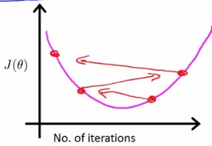
working correctly: If gradient descent is working then J(θ) should decrease after every iteration
convergence: 收敛是指每经过一次迭代，J(θ)的值都变化甚小。
choose α
1. When to use a smaller α
  - If J(θ) is increasing, see below picture
  - If J(θ) looks like a series of waves, decreasing and increasing again
  - But if α is too small then rate is too slow
2. Try a range of α values
  - Plot J(θ) vs number of iterations for each version of alpha
  - Go for roughly threefold increases: 0.001, 0.003, 0.01, 0.03. 0.1, 0.3

Features and polynomial regression

Can create new features

如何选择 features 和表达式尤为关键，例如房价与房子的长，房子的宽组成的表达式就会麻烦很多，若将房子的长乘以房子的宽得出面积，则有房价与房子面积的表达式，将会更容易拟合出房价的走势。

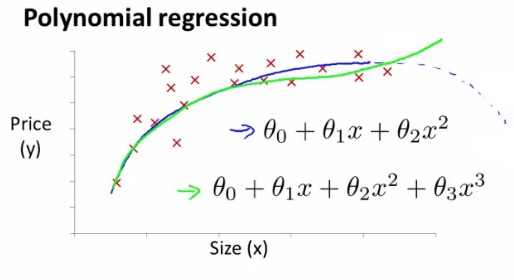
Polynomial regression

例如房价的走势，如下图，横坐标 x 为房子的面积，纵坐标为房价，使用一元二次的方程，会得出下图的蓝色曲线。容易得到房价今后会有一个下降的过程，可实际上房价是不会随着面积的增大而下降的。所以需要重新选定 Polynomial regression，可以改为使用一元三次的方程或者使用平凡根的方程。

所以选择合适的 Features 和 Polynomial regression 都非常重要。

Normal equation 求解多变量线性回归

Normal equation

举例说明，假设 J(θ) 是一元二次方程，如：J(θ)=a$θ^2$+bθ+c，则令 $\frac{d}{dθ}J(θ)=2aθ+b=0$ 即可，求出最终的 θ 则得到了线性回归方程，可以预测出今后的 y 值。

更普遍地，当 θ 是一个 n+1 维的向量时，θ $\in$ $R^{n+1}$，则 cost function 如下：

$J(θ_0, θ_1, ...,θ_n) = \frac1{2m}\sum_{i=1}^{m}{(h_θ(x^{(i)}) - y^{(i)})^2}$

只需要令：

$\frac\partial{\partial θ_j}J(θ_0, θ_1, ...,θ_n) = ... = 0 $$，其中 j = 0,1,2,...,n 设 X 代表训练集的 features 的值的矩阵，y 代表训练集的结果的值的矩阵，假设训练集数量为 m, features 个数为 n, 则 X 为 (m\*n) 的矩阵，y 为 (m\*1) 的矩阵，可以推导出求 θ 向量的公式如下： $$θ = (X^TX)^{-1}X^Ty$

Gradient descent Vs Normal equation

Gradient descent

Need to chose learning rate
Needs many iterations - could make it slower
Works well even when n is massive (millions)
Better suited to big data
What is a big n though: 100 or even a 1000 is still (relativity) small, If n is 10000 then look at using gradient descent
适用于线性回归会逻辑回归

Normal equation

No need to chose a learning rate
No need to iterate, check for convergence etc.
Normal equation needs to compute $(X^TX)^{-1}$
- This is the inverse of an n x n matrix
- With most implementations computing a matrix inverse grows by O(n3), So not great
Slow of n is large, Can be much slower
仅适用于线性回归

局部加权线性回归

局部加权回归(locally weighted regression)简称 loess，其思想是，针对对某训练数据的每一个点，选取这个点及其临近的一批点做线性回归；同时也需要考虑整个训练数据，考虑的原则是距离该区域越近的点贡献越大，反之则贡献越小，这也正说明局部的思想。其 cost function 为：

$J(\theta) = \sum_{i=1}^{m} w^{(i)}( y^{(i)}-\theta^Tx^{(i)} )^2$

其中

$w^{(i)} = exp (-\frac{(x^{(i)}-x)^2}{\tau^2})$

$w^{(i)}$的形式跟正态分布很相似，但二者没有任何关系，仅仅只是便于计算。可以发现，$x^{(j)}$ 离 $x^{(i)}$ 非常近时，${w^{(i)}_j}$ 的值接近于1，此时 j 点的贡献很大，当 $x^{(j)}$ 离 $x^{(i)}$ 非常远时，${w^{(i)}_j}$ 的值接近于 0，此时 j 点的贡献很小。

$\tau^2$ 是波长函数(bandwidth)，控制权重随距离下降的速度，τ 越小则 x 离 $x^{(i)}$ 越远时 $w^{(i)}$ 的值下降的越快。

所以，如果沿着 x 轴的每个点都进行局部直线拟合，那么你会发现对于这个数据集合来说，局部加权的预测结果，能够最终跟踪这条非线性的曲线。

但局部加权回归也有其缺点：

每次对一个点的预测都需要整个数据集的参与，样本量大且需要多点预测时效率低。提高效率的方法参考 Andrew More’s KD Tree
不可外推，对样本所包含的区域外的点进行预测时效果不好，事实上这也是一般线性回归的弱点

对于线性回归算法，一旦拟合出适合训练数据的参数θ，保存这些参数θ，对于之后的预测，不需要再使用原始训练数据集，所以是参数学习算法。

对于局部加权线性回归算法，每次进行预测都需要全部的训练数据（每次进行的预测得到不同的参数θ），没有固定的参数θ，所以是非参数算法(non-parametric algorithm)。

Reference

http://www.holehouse.org/mlclass/04_Linear_Regression_with_multiple_variables.html